In my last column, we discussed the Modifiable Unit Area Problem, and how it can affect analysis of spatial data. This column discusses the related issue of spatial autocorrelation, which can have similarly negative effects on decision making if ignored. We will give examples of spatial autocorrelation, discuss how to test for it, and examine its effects.

What is Spatial Autocorrelation?

When analyzing data statistically, we are used to the assumption of independence between measurements. For example, imagine that you and a friend are playing monopoly. Rolling a 12 on a pair of dice on your turn does not affect the probability of your friend rolling a 12 during his turn. Standard statistical techniques often assume independence. This simplifies techniques, and is usually a reasonable assumption. Everything from gambling odds calculation to scientific experiment design assumes that multiple results are independent, and is often specifically built so that this assumption is not violated (as anyone who has been kicked out of Vegas for card counting knows). However, this assumption does not work for spatial data.

The entire reason why geographic analysis is so common is that examining something allows you to draw inferences about its neighbors. This works because spatial events are not generally independent of each other. For example, intersections near an especially dangerous intersection are more likely than average to be dangerous themselves, due to commonly shared phenomena like amount of traffic and bad design elements. This phenomenon is known as spatial autocorrelation, and it is generally stated in the following form, which is known as Tobler’s first law: “Everything is related to everything else, but near things are more related than distant things.”  In other words, common factors shared between items, events, and locations that are near each other often result in a high correlation between values of the attributes of those things. The data below provides a useful example of this:

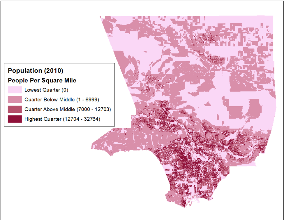
Figure 1: Clustering of values for areas

The map above shows the population density for each census block in Los Angeles county. Two trends are apparent here. The first is that population densities cluster in specific parts of the county. The second is that specific spatial features, such as parks, airports, and rivers, will “force” a low population density, causing the population density map to effectively outline those features. This is most apparent with the mountain range in the middle of the city, which is visible as a large area of low population between two densely populated areas.  These effects may seem obvious at first glance (because “common sense” accounts for spatial autocorrelation), but they invalidate many statistical techniques. For example, it is common practice during statistical investigations to perform tests on a sample, which uses the fact that a sample consisting of independent observations of a population tends to have the same distribution of values as the whole population. However, spatial autocorrelation makes it much harder to independently select sample observations. This is because observations that are near each other are not independent if the data are spatially autocorrelated. This is shown by the map below.

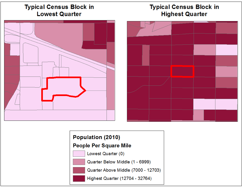
Figure 2: Examples of clustering

This figure is an excellent example of how Spatial Autocorrelation can affect the distribution of values for local samples. Both census blocks above are surrounded by blocks in the same quarter, even though you would expect values to be evenly distributed. This is a standard feature for highly autocorrelated data. Note how the thin object representing the freeway at the top of the left-hand image always has zero density.

It is also worth noting that Spatial Autocorrelation comes in both positive and negative varieties. Positive autocorrelation is where like values “clump” as noted above. Negative Autocorrelation is where there is less clumping than would be observed if the values were randomly redistributed. Perfect negative autocorrelation means that the values are in a “chessboard” arrangement, with dissimilar values alternating.

How do you detect Spatial Autocorrelation?

Although Spatial Autocorrelation is often detectable visually as a “clumping” effect, this is not always the case (especially because some “clumping” may be found among non-correlated data). The primary method for detecting Spatial Autocorrelation is a measurement known as Moran’s I, which varies between 1 (perfect positive autocorrelation) and -1 (perfect negative autocorrelation). A value of zero indicates no autocorrelation. Moran’s I requires that a “spatial weights matrix” be determined in some way for each point, representing how adjacent each other point is to that point. This matrix can be determined in a variety of ways, including several types of binary or inverse distance weighting. This is then plugged into the equation for Moran’s I, which determines the level of autocorrelation between adjacent values using this matrix. A P value can also be determined, in order to determine whether the observed value is the result of random chance. A useful way to determine what spatial scale the autocorrelation operates on is to use Moran’s I multiple times with different spatial weights matrices. Many software suites have additional features that allow the user to examine autocorrelation, such as the semi-variogram.

How can Spatial Autocorrelation be dealt with?

When performing an analysis of spatial data, it is a good idea to think about the data and visually inspect it. The next step is to apply Moran’s I and any other tools that your software package offers in order to see whether your dataset is spatially autocorrelated, and if so, how. If spatial autocorrelation is found, it pays to be very careful about what statistical methods you use. Check the assumptions behind each method to make sure that it does not assume independence. Spatial Autocorrelation should also be kept in mind when checking other people’s work. If a value of I or other measure is not given, yourself it is especially important to think about whether Spatial Autocorrelation is likely to be an issue. Often, this is not obvious. For example, a survey that obtains respondents by asking questions at a street corner is likely to have hidden Spatial Autocorrelation issues, because people with similar characteristics are likely to frequent whatever amenities are located near that corner. These steps should help comprehensively deal with spatial autocorrelation, so that it does not accidently taint analytical results.

Sources:

O’sullivan, David,  and David Unwin. “Area Objects and Spatial Autocorrelation.” Geographic Information Analysis. Hoboken: John Wiley & Sons, 2010. 187-213. Print.

Biography:

Efram Stone is a dual Masters student in the Transportation Engineering and Transportation Planning programs at the University of Southern California who is also working on a GIS Certificate there. Efram’s interest in transportation began at a young age when he attended elementary school next to a major infrastructure project, and has continued unabated since. Efram plans to graduate in May, 2017. He can be reached at [email protected].